class: center, middle, inverse, title-slide # Introductory statistics ### Nathalie Vialaneix & Sandrine Laguerre ### Toulouse, March 14-16 – 2022 --- <!-- Section 1: introduction, definition, types of variables --> ## An elementary map of statistics .center[<img src="img/statistics-map.png" height="500">] --- ## An elementary map of statistics .center[<img src="img/statistics-map-filled.png" height="500">] --- ## Before you start: tidy your data! .left[<img src="img/real-data.png" height="300">] --- ## Before you start: tidy your data! .left[<img src="img/real-data.png" height="300"> <img src="img/clean-data.png" height="300"> <img src="img/tidy_data.png" width="350">] **clean data**: one sample in each row, one variable in each column, one value in each cell .center[“Like families, tidy datasets are all alike but every messy dataset is messy in its own way.“] <font size="3">Hadley Wickham (2014) Tidy Data. Journal of Statistical Sofware, 59(10).</font> --- ## Types of variables * numeric (discrete or continuous) * non numeric (ordered or not) <img src="img/warning.png" height="50"> how things are encoded! .right[<img src="img/clean-data.png" height="350">] --- class: center, inverse, middle <!-- Section 2: univariate statistics (and graphics) --> ## Univariate statistics --- ## Statistics (e.g., numerical characteristics) ### Purpose summarize a series of values by one numeric value -- ### central characteristics *indicateurs de tendance centrale* ### dispersion characteristics *indicateurs de dispersion* --- ## Central characteristics - **Mean** (**Moyenne**): sum of the observed values divided by the number of observations: `\(\overline{X} = \frac{1}{n} \sum_{i=1}^n x_i\)` - **Median** (**Médiane**): value that splits the sample into two subsamples with equal sizes - **Mode** (**Mode**): most frequently observed values - **Quartiles** (**Quartiles**): 3 values that split the sample into 4 equal size subsamples - **Deciles** (**Déciles**): 9 values that split the sample into 10 equal size subsamples - **Percentiles** (**Percentiles**): 99 values that split the sample into 100 equal size subsamples - **Quantiles** (**Quantiles**): generalize the others --- ## Never heard of percentiles? .center[<img src="img/carnet-sante.png" height="500">] --- ## Mean and median: the mean is not robust! How to increase the mean salary in a company? -- * increase all salaries of `\(x\)`\% * increase the salary of the most well paid person * suppress a few jobs with low salaries --- ## Are central characteristics enough? <!-- --> 10 marks for 5 students: same mean, same median --- ## Dispersion characteristics * **variance**: average squared distance to the mean `\(\mbox{Var}(X) = \frac{1}{n} \sum_{i=1}^n (x_i - \overline{X})^2\)` and **standard deviation** (*écart type*): `\(\sigma_X = \sqrt{\mbox{Var}(X)}\)` -- <br> <br> * **range** (*étendue*): difference between the largest and the smallest values * **inter-quartile range** (*écart inter-quartile*): difference between the 1st and the 3rd quartiles (half of the observations lie between these two quantities) --- ## A few properties for the standard deviation * positive (or null if all the observations have the same value) * does not change when values are translated * sensible to extreme values (like the mean) * expressed in the same unit than the original variable (like the mean) <br> <br> -- **Consequences** * mean and standard deviation can be added (confidence interval) * they can also be divided: `\(\mbox{CV}(X) = \frac{\sigma_X}{\overline{X}}\)` (*coefficient de variation*) can be used to compare the respective variability of two series --- ## Example of the impact of variability « **Les filles brillent en classe, les garçons aux concours** *LE MONDE | 07.09.09 - Article paru dans l'édition du 08.09.09. Philippe Jacqué* Elles obtiennent de meilleurs résultats en cours de scolarité, mais réussissent moins bien les concours des meilleures grandes écoles que les hommes. [...] Pour vérifier [cette hypothèse], trois économistes - Evren Örs, professeur à HEC, Eloïc Peyrache, directeur d'HEC, et Frédéric Palomino, ancien de l'école parisienne et actuel professeur associé à l'Edhec Lille - ont étudié à la loupe les résultats obtenus entre 2005 et 2007 au concours d'admission en première année d'HEC, une des écoles de management les plus réputées. [...] « D'un point de vue technique, il semble que la structure du concours HEC crée d'avantage d'hétérogénéité chez les hommes que chez les femmes », estime M. Peyrache. Si, « en moyenne », les performances des hommes et des femmes sont similaires, « les notes des femmes sont concentrées autour de la moyenne, tandis que celles des hommes sont très dispersées avec beaucoup de très bonnes notes et de très mauvaises. Mécaniquement, quand on sélectionne les 380 premiers résultats, on a un peu plus d'hommes ». --- ## Standard modifications of data * **binarization of a numeric variable** (*discrétisation*): transform a numeric variable into a factor by: <ul> <li>creating intervals of equal width</li> <li>creating intervals of equal number of observations (<em>how to do that?</em>)</li> <li>other...</li> </ul> -- <br> <br> Which solution sounds the best? What are the advantages/drawbacks of such a transformation? --- ## Standard modifications of data * **centering and scaling (to unit variance)** (*centrage et reduction*), often called **Z-score**: <ul> <li>centering: removing the mean</li> <li>scaling: dividing by the standard deviation</li> </ul> `\(z_i = \frac{x_i - \overline{X}}{\sigma_X}\)` <br> After centering and scaling, the mean of the variable is 0 and its standard deviation is 1. <!-- --> --- ## Log transformations <!-- --> * useful for asymetric distribution to make the variable fit a Gaussian distribution (after transformation) `\(\Rightarrow\)` often performed before tests * useful for ratios (because a value twice or half the other have the same log with opposite signs) * for `\(p\)`-values, `\(\log_{10}\)` is often used * most frequent logs: <ul> <li> `\(y = \log_2(x) \Leftrightarrow x = 2^y\)` </li> <li> `\(y = \log_{10}(x) \Leftrightarrow x = 10^y\)` </li> <li> `\(y = \ln(x) \Leftrightarrow x = \exp(y)\)` </li> </ul> --- ## Other transformations * compute ratios * normalization * other functions ( `\(\sqrt{.}\)` , ...) --- ## Display a series of values with a chart ### In theory, a graphic should: * show the data * help looking at it and understanding the data structure somehow * avoid data distorsion * plot many data in a simple way **References** * Edward Tufte (1983) *The Visual Display of Quantitative Information*, Graphics Press. * http://r-graph-gallery.com/ --- ## Common graphics for univariate analyses The type of chart depends on... -- .. the variable type: * factors: -- <ul> <li>pie charts</li> <li>bar charts</li> <li>spider charts</li> <li>...</li> </ul> .center[<img src="img/pie.png" height="200"> <img src="img/bar.png" height="200"> <img src="img/spider.png" height="200">] --- ## Common graphics for univariate analyses The type of chart depends on... .. the variable type: * numeric: -- <ul> <li>histograms / density plots</li> <li>boxplot / violin plots</li> <li>...</li> </ul> .center[<img src="img/histogram.png" height="150"> <img src="img/density.png" height="150"> <img src="img/boxplot.png" height="150"> <img src="img/violin.png" height="150">] --- ## Boxplots? .center[<img src="img/boxplot_explanation.png" height="500">] --- ## Most frequently seen mistakes Try to keep the lie factor close to 1: `\(\frac{\textrm{effect size on graphic}}{\textrm{effect size in data}}\)` * *Which category is the most frequent between C and A?* .center[<img src="img/pie_ok.png" height="200"> <img src="img/pie_3d.png" height="200">] --- ## Most frequently seen mistakes Try to keep the lie factor close to 1: `\(\frac{\textrm{effect size on graphic}}{\textrm{effect size in data}}\)` * *Are the differences between the categories important?* .center[<img src="img/bars_distorted.png" height="400">] --- ## Hum, hum... Try to keep the lie factor close to 1: `\(\frac{\textrm{effect size on graphic}}{\textrm{effect size in data}}\)` .center[<img src="img/hum_chart_1.png" height="500">] --- ## Hum, hum... Try to keep the lie factor close to 1: `\(\frac{\textrm{effect size on graphic}}{\textrm{effect size in data}}\)` .center[<img src="img/hum_chart_2.png" height="500">] --- ## Hum, hum... Try to keep the lie factor close to 1: `\(\frac{\textrm{effect size on graphic}}{\textrm{effect size in data}}\)` .center[<img src="img/hum_chart_3.png" height="250">] **Une année de présidence Hollande en chiffres** by http://www.lemonde.fr/politique/visuel/2013/05/06/une-annee-de-presidence-hollande-en-chiffres_3170215_823448.html Comments by readers: * « Vous êtes vous interrogés sur le contenu de votre infographie ? sur les polices de caractères utilisées ? Sur les zooms ? Où est l'objectivité et le factuel ? » --- ## Hum, hum... Try to keep the lie factor close to 1: `\(\frac{\textrm{effect size on graphic}}{\textrm{effect size in data}}\)` .center[<img src="img/hum_chart_3.png" height="250">] Comments by readers: * « Merci de corriger votre 1er graphique, qui fait croire à une augmentation du chômage plus lente sur la dernière période, après une augmentation plus rapide sur la période précédente, ce qui est l'EXACT CONTRAIRE de la réalité : Février 08 à Avril 11 (38 mois) : 2 696 300-1 983 100 = 713 200 / 38 mois = 18 768 par mois. Avril 11 à Mai 12 (13 mois) : 2 927 600-2 696 300 = 231 300 / 13 mois = 17792 par mois (976 de -). Mai 12 à Mars 13 (10 mois) : 3 224 600-2 927 600 = 297000 / 10 mois = 29 700 par mois (11 908 de +). » --- class: center, inverse, middle <!-- Section 3: bivariate statistics (and graphics) --> ## Bivariate statistics --- ## Standard numerical summaries * factor vs factor -- ### contingency tables .center[<img src="img/contingency_table.png" height="200">] ... with variants (row / column profiles, percentages, ...) --- ## Standard numerical summaries * factor vs factor ### Cramer's `\(V\)` (also linked to `\(\phi\)` coefficient) `\(V = \sqrt{\frac{\chi^2}{n \times \min(\textrm{nrow} - 1,\ \textrm{ncol} - 1)}}\)` * `\(0 \leq V \leq 1\)` * `\(V = 0 \Leftrightarrow X\)` and `\(Y\)` are perfectly independent * `\(V = 1 \Leftrightarrow\)` knowing the value of `\(X\)` (resp. `\(Y\)`), you know the value of `\(Y\)` (resp. `\(X\)`) -- /!\ **Cramer's `\(V\)`**: * is a **descriptive** statistics (does not provide any evidence of meaningful correlation) * tends to be biased (overestimates the strength of the correlation) --- ## Standard numerical summaries * numeric vs numeric -- ### covariance `\(\mbox{Cov}(X,Y) = \frac{1}{n} \sum_{i=1}^n (x_i - \overline{X}) (y_i - \overline{Y})\)` .center[<img src="img/covariance.png" height="200">] sum of negative green areas and positive blue areas scales as the product of the variable units `\(\Rightarrow\)` coefficient of correlation --- ## Coefficient of correlation <ul> <li><strong>Pearson correlation coefficient</strong>: `\(r(X,Y) = \frac{\mbox{Cov}(X,Y)}{\sigma_X \sigma_Y}\)`</li> </ul> ranges between -1 and 1, with `\(\pm 1\)` indicating perfect linear correlations<br> positive when the two variables vary in the same direction<br> is sensitive to outliers and can only detect linear relations -- <ul> <li><strong>Spearman correlation coefficient</strong>: Pearson correlation for the <strong>ranks</strong></li> </ul> ranges between -1 and 1, with `\(\pm 1\)` indicating identical or opposite ranks between the two variables<br> positive when the two variables vary in the same direction<br> is not sensitive to outliers and can detect any monotonic relation --- ## Correlation: examples ``` ## `geom_smooth()` using formula 'y ~ x' ``` 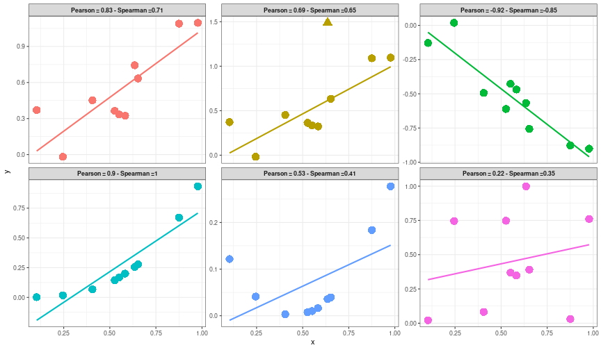<!-- --> --- ## Do not over-interpret the correlation coefficient! ``` ## `geom_smooth()` using formula 'y ~ x' ``` <!-- --> With `\(n=50\)` observations the correlation coefficient is significatively different from 0 at approximately 0.27 (for a 5% risk). --- ## Correlation `\(\neq\)` Causality! Spurious correlations: http://www.tylervigen.com/spurious-correlations .center[<img src="img/divorce-vs-margarine.png" height="450">] --- ## Correlation `\(\neq\)` Causality! Spurious correlations: http://www.tylervigen.com/spurious-correlations .center[<img src="img/drowning-vs-nicholascage.png" height="450">] --- ## ... an often forgotten fact! ### Faut-il manger du chocolat pour avoir des prix Nobel ? .left[<img src="img/nobel_vs_chocolat.jpg" height="150"> *©REUTERS/Denis Balibouse*] La revue médicale New England Journal of Medicine vient de publier une étude qui fait le lien entre une forte consommation de chocolat et l'attribution des Nobel. New England Journal of Medicine, hebdomadaire américain, publié depuis 1812, est considéré comme la revue médicale la plus prestigieuse. [...] Le docteur Franz Messerli, de l'université Columbia à New York et auteur de l'étude, explique « qu"il y a une corrélation significative surprenante entre la consommation de chocolat per capita et le nombre de lauréats du Nobel pour dix millions d'habitants dans un total de 23 pays ». [...] Seule exception de l'étude : la Suède. Les habitants ne consomment « que » 6,4 kilos de chocolat par an et par personne pour un total de 32 Nobel. Qu'à cela ne tienne, pour les chercheurs il s'agirait d'un simple favoritisme du comité Nobel. Si une corrélation est montrée pour les pays, l'étude ne dit rien en revanche sur le niveau de consommation individuel de chocolat des lauréats du Nobel. --- ## ... but: ### Le chocolat engendre des tueurs en série *23/11/2012 | Mise à jour: 11:12 Réactions (24) Par Hayat Gazzane* http://plus.lefigaro.fr/lien/le-chocolat-engendre-des-tueurs-en-serie-20121123-1589103 Des chercheurs britanniques se sont amusés à démonter l'étude de Franz Messerli qui établit une corrélation forte entre consommation de chocolat et prix Nobel. En utilisant la même méthodologie, ils arrivent à prouver que les pays où l'on mange beaucoup de chocolat sont aussi ceux qui engendrent le plus de serial killer et d'accidents de la route (étude en anglais). ### and also « la statistique expliquée à mon chat » https://www.youtube.com/watch?v=aOX0pIwBCvw --- ## Confounding variable: the Simpson's paradox ### Shark attacks are correlated with ice cream sales -- .center[<img src="img/sharks_vs_icecream.png" height="500">] --- ## How can that be handled? <img src="img/needs-partialcor.png" height="150"> If you know the potential confounding variables, use **partial correlation**! ```r set.seed(2807) x <- rnorm(100) y <- 2*x + 1 + rnorm(100,0,0.1) z <- -2*x + 2 + rnorm(100,0,0.1) cor(x,y); cor(x,z); cor(y,z) ``` ``` ## [1] 0.9988261 ``` ``` ## [1] -0.998756 ``` ``` ## [1] -0.9980506 ``` --- ## How can that be handled? <img src="img/needs-partialcor.png" height="150"> If you know the potential confounding variables, use **partial correlation**! ```r cor(lm(x~z)$residuals, lm(y~z)$residuals) ``` ``` ## [1] 0.6481373 ``` ```r cor(lm(x~y)$residuals, lm(z~y)$residuals) ``` ``` ## [1] -0.6208908 ``` ```r cor(lm(y~x)$residuals, lm(z~x)$residuals) ``` ``` ## [1] -0.1933699 ``` --- ## Standard numerical summaries * numeric ( `\(X\)` ) vs factor ( `\(Y \in \{1, ..., K\}\)` ) -- ### correlation ratio `\(Y\)` can be seen as a variable that defines *groups of individuals* **within-group variance**: `\(\mbox{Var}_{\textrm{intra}} = \frac{1}{n} \sum_{k=1}^K n_k \sigma_{X,k}^2\)` in which `\(n_k\)` is the number of individuals for which `\(Y = k\)` and `\(\sigma_{X,k}^2\)` is the variance of `\(X\)` for individuals for which `\(Y=k\)` *average variance of `\(X\)` within the groups defined by `\(Y\)` * -- **between-group variance**: `\(\mbox{Var}_{\textrm{inter}} = \frac{1}{n} \sum_{k=1}^K n_k (\overline{X}_{k} - \overline{X})^2\)` in which `\(\overline{X}_{k}\)` is the mean of `\(X\)` for individuals for which `\(Y=k\)` *variance between means of `\(X\)` within the groups defined by `\(Y\)` * --- ## Standard numerical summaries * numeric ( `\(X\)` ) vs factor ( `\(Y \in \{1, ..., K\}\)` ) -- ### correlation ratio It turns out that: `\(\mbox{Var}_{\textrm{intra}} + \mbox{Var}_{\textrm{inter}} = \mbox{Var}(X)\)` -- The correlation ratio is defined as: `\(\eta(X|Y) = \sqrt{\frac{\mbox{Var}_{\textrm{inter}}}{\mbox{Var}_{\textrm{X}}}}\)` *proportion of the variance explained by the groups* -- **Properties**: <ul> <li>between 0 and 1</li> <li>equal to 1 if and only if the individuals within a given group all have the same value for `\(X\)` for all groups</li> <li>equal to 0 if and only if the average values for the groups are exactly identical</li> </ul> --- ## Common graphics for bivariate exploration The type of chart depends on... .. the variable types: * a numeric variable vs a factor: -- <ul> <li>numeric charts but made parallel: superimposed histograms / density plots, parallel boxplot / violin plots...</li> <li>dot plots</li> </ul> .center[<img src="img/parallel_histograms.png" height="150"> <img src="img/parallel_densities.png" height="150"> <img src="img/boxplot.png" height="150"> <img src="img/violin.png" height="150"> <img src="img/dot_plot.png" height="150">] --- ## Common graphics for bivariate exploration The type of chart depends on... .. the variable types: * two factors: -- barplots (side-by-side, stacked, ...) .center[<img src="img/barplot_stacked.png" height="250">] --- ## Common graphics for bivariate exploration The type of chart depends on... .. the variable types: * two numeric variables: -- scatterplot or scatterplot matrices for more than two variables... .center[<img src="img/scatterplot.png" height="250"> <img src="img/scatterplot-matrix.png" height="250">] --- class: center, inverse, middle <!-- Section 4: inference (tests) --> ## Inference (tests) --- ## Inference .center[**From a sample, obtain general conclusions (with a control of the error) on the whole population from which the sample has been taken.**] <br> <br> * **confidence interval**: from the sample, define an interval in which the average value for a given variable is likely to be <br> <br> * **statistical test**: from the observations made on a sample, can we invalidate an assumption made on the whole population? --- ## Different steps in hypothesis testing 1. formulate an **hypothesis `\(H_0\)` **: .center[ `\(H_0\)` : the average count for gene `\(g\)` in the control samples is the same than the average count in the treated samples] which is tested against an alternative `\(H_1\)`: the average count for gene `\(g\)` in the control samples is different from the average count in the treated samples .center[<img src="img/samples-counts-1.png" height="300">] --- ## Different steps in hypothesis testing 1. formulate an **hypothesis `\(H_0\)` ** 2. **from observations**, calculate a **test statistics** (*e.g.*, the standardized difference between means in the two samples) .center[<img src="img/samples-summary-1.png" height="300">] --- ## Different steps in hypothesis testing 1. formulate an **hypothesis `\(H_0\)` ** 2. **from observations**, calculate a **test statistics** 3. find the **theoretical distribution of the test statistics under `\(H_0\)` ** .center[<img src="img/theoretical-dist.png" height="300">] --- ## Different steps in hypothesis testing 1. formulate an **hypothesis `\(H_0\)` ** 2. **from observations**, calculate a **test statistics** 3. find the **theoretical distribution of the test statistics under `\(H_0\)` ** 4. deduce the probability that the observations occur under `\(H_0\)`: this is called the **p-value** .center[<img src="img/theoretical-dist-sample-1.png" height="300">] --- ## Different steps in hypothesis testing 1. formulate an **hypothesis `\(H_0\)` ** 2. **from observations**, calculate a **test statistics** 3. find the **theoretical distribution of the test statistics under `\(H_0\)` ** 4. deduce the probability that the observations occur under `\(H_0\)`: this is called the **p-value** 5. conclude: if the p-value is low (usually below `\(\alpha=5\)`\% as a convention), `\(H_0\)` is unlikely: we say that " `\(H_0\)` is rejected". We have that: .center[<font size="6"> `\(\alpha = \mathbb{P}_{H_0} (H_0\mbox{ is rejected})\)` </font>] --- ## Statistics premises in short <br> .center[<font size="6"> `\(H_0 \Rightarrow\)` theoretical distribution for a given test statistics</font>] <br> <br> .center[**then**] <br> <br> .center[<font size="6"> observed value has a low probability under the theoretical distribution `\(\Rightarrow\)` `\(H_0\)` is unlikely] --- ## Summary of the possible decisions .center[<table> <tr> <td><img src="img/samples-summary-1.png" height="200"></td> <td> </td> <td><img src="img/samples-summary-2.png" height="200"></td> </tr> <tr> <td><img src="img/theoretical-dist-sample-1.png" height="200"></td> <td> </td> <td><img src="img/theoretical-dist-sample-2.png" height="200"></td> </tr> <tr> <td>can not reject `\(H_0\)` </td> <td> </td> <td>reject `\(H_0\)` </td> </tr> </table>] --- ## Types of errors in tests .center[<img src="img/error_types.png" height="400">] `\(\mathbb{P}(\mbox{Type I error}) = \alpha\)` (risk) <br> `\(\mathbb{P}(\mbox{Type II error}) = 1-\beta\)` with `\(\beta\)` : power --- ## A few remarks on p-values * The p-value is the probability to observe the current value of the test statistics or a more extreme one under the null hypothesis <br> <br> Hence: <br> .center[<font size="6">the smaller the p-value, the smaller the risk to make an error while rejecting `\(H_0\)` </font>] <br> <br> <br> -- .center[<font size="6">results of tests are not just white/black: the p-value gives a degree of confidence in the conclusion</font>] -- * decision is not symmetric: rejecting `\(H_0\)` means that the error risk is under control (the test is said **significant**) while not rejecting `\(H_0\)` provides no guarantee on the error risk ( `\(1-\beta\)` ; the test is said **not significant**) --- ## Controlling `\(\alpha\)` AND `\(\beta\)` The only way to simultaneously control `\(\alpha\)` and increasing `\(\beta\)` is to **increase the sample size**. -- ### Basics on computing sample size Facts on `\(\beta\)` : `\(\beta\)` increases when: * `\(\alpha\)` increases * the sample size increases * the effect size increases (*i.e.*, the alternative hypothesis becomes more distinct from the null hypothesis) `\(\Rightarrow\)` defining *a priori* values for `\(\alpha\)`, `\(n\)` and the effect size can be used to give an estimate of the power (and reciprocally, fixing a power can be used to target a relevant sample size) --- ## Example of a sample size computation Extract of `?power.t.test`: <img src="img/help_power.png" height="500"> --- ## Example of a sample size computation ```r power.t.test(n = 25, delta = 1, sd = 1, sig.level = 0.05, power = NULL) ``` ``` ## ## Two-sample t test power calculation ## ## n = 25 ## delta = 1 ## sd = 1 ## sig.level = 0.05 ## power = 0.9337076 ## alternative = two.sided ## ## NOTE: n is number in *each* group ``` ```r power.t.test(n = NULL, delta = 1, sd = 1, sig.level = 0.05, power = 0.9) ``` ``` ## ## Two-sample t test power calculation ## ## n = 22.0211 ## delta = 1 ## sd = 1 ## sig.level = 0.05 ## power = 0.9 ## alternative = two.sided ## ## NOTE: n is number in *each* group ``` --- ## What about confidence intervals? 1. **from observations**, calculate a **test statistics** `\(S_n\)` 2. find the **theoretical distribution of the test statistics** 3. using this theoretical distribution, find an interval, IC, with a high probability ( `\(1-\alpha\)` ) to find the test statistics (as defined in the population) in: $$ \mathbb{P}(S_n \in \textrm{IC}) \geq 1-\alpha $$ <img src="img/intervalle-confiance.jpg" alt="IC" width = "500" /> Testing `\(H_0\)`: " `\(S\)` is equal to 0" `\(\Leftrightarrow\)` `\(0 \in \textrm{IC}\)` --- ## Why is the Gaussian (normal) distribution so central in many tests / confidence intervals? .center[<img src="img/galton_box.png" height="300"> <img src="img/galton_box_2.jpg" height="300">] --- ## Tests for one variable ### parametric tests **comparison of a mean to a given value ( `\(H_0\)` : `\(\overline{X}\)` is equal to 0): `\(t\)` test (Student)** <ul> <li> `\(X\)` is supposed to follow a Gaussian law (with unknown variance) </li> <li> the test statistics is: `\(T = \frac{\overline{X} - 0}{\sigma_X / \sqrt{n}}\)` </li> <li> under the null hypothesis, the theoretical distribution is the Student law with `\(n-1\)` degrees of freedom</li> <li> accepting the null hypothesis is equivalent to have the target tested value (0 in the example above) included in the confidence interval for `\(X\)`</li> </ul> -- ### non parametric tests **adequation of the distribution of `\(X\)` to a given distribution (very often, the Gaussian distribution)** <ul> <li>no assumption on the distribution of `\(X\)` </li> <li>median: Wilcoxon test</li> <li>normality: Shapiro-Wilk</li> <li>any theoretical distribution: Kolmogorov-Smirnov, `\(\chi^2\)` (compare observed frequencies in intervals with theoretical frequencies)</li> </ul> --- ## Tests with two variables ### factor vs factor independence between the two variables `\(\chi^2\)` test (non parametric) of a contingency table or Fisher exact test (non parametric but limited to small contingency tables and sample sizes) **Titanic (males, adults)**: .center[ <img src="img/titanic_table.png" height="100"> <img src="img/titanic_profiles.png" height="100"> ] .center[ contingency table row profiles ] Independence means the same level of survival whatever the class (for instance, 20% of survival whatever the class). --- ## Tests with two variables ### numeric variable vs numeric variable test for correlation/association between two numeric variables <ul> <li> `\(X\)` and `\(Y\)` are Gaussian: Pearson correlation (parametric / only for linear relations)</li> <li> otherwise: Spearman correlation (non parametric / not restricted to linear relations)</li> </ul> -- ### numeric variable vs factor factor can be seen as a group variable `\(\Rightarrow\)` these are called comparison of `\(K\)` samples tests can be for **paired** samples or **unpaired** samples --- ## Comparison between samples `\(K = 2\)` ### Comparison of the distribution of `\(X\)` in group 1 and in group 2 (unpaired samples) Kolmogorov-Smirnov -- ### Comparison of a central characteristic of `\(X\)` in group 1 and in group 2 .center[<img src="img/table-comptest-2.png" height="250">] --- ## Comparison between samples `\(K = 2\)` ### Comparison of the variance / dispersion of `\(X\)` in group 1 and in group 2 Fisher test ( `\(K=2\)` ): `\(X\)` is supposed to be Gaussian (parametric) Siegel-Tukey test (non parametric, can be used with an ordinal variable) --- ## Comparison between samples `\(K \geq 2\)` ### Comparison of a central characteristic of `\(X\)` in groups .center[<img src="img/table-comptest-2more.png" height="100">] -- ### Comparison of the variance / dispersion of `\(X\)` in groups Levene (also Brown–Forsythe) or Bartlett tests (parametric) --- ## Need help? GIYF: choose a statistics test .center[<img src="img/choose_test.jpg" height="300">] --- ## A last note on how data must be prepared for paired / unpaired tests ### not paired ``` ## extra group ID ## 9 0.0 A 9 ## 12 0.8 B 2 ## 6 3.4 A 6 ## 15 -0.1 B 5 ## 18 1.6 B 8 ## 7 3.7 A 7 ``` ### paired ``` ## before after ## 1 200.1 392.9 ## 2 190.9 393.2 ## 3 192.7 345.1 ## 4 213.0 393.0 ## 5 241.4 434.0 ## 6 196.9 427.9 ``` --- class: center, inverse, middle <!-- Section 5: Inference (linear models) --> ## Inference (linear models) --- ## Linear regression, linear models **Case where `\(Y\)` (numeric) is explained by one or several explanatory variables `\(X_j\)` (all numeric)**: $$ Y = a + b X + \epsilon $$ **Very important remark**: Testing `\(H_0:\ b=0\)` is exactly equivalent to testing `\(\textrm{Cor}(X,Y) = 0\)` (Pearson correlation test)! <!-- --> $$ Y = a + b_1 X_1 + b_2 X_2 + \epsilon $$ --- ## Linear regression `\(Y = a + b X + \epsilon\)` ``` ## ## Call: ## lm(formula = Sepal.Width ~ Petal.Width, data = iris) ## ## Residuals: ## Min 1Q Median 3Q Max ## -1.09907 -0.23626 -0.01064 0.23345 1.17532 ## ## Coefficients: ## Estimate Std. Error t value Pr(>|t|) ## (Intercept) 3.30843 0.06210 53.278 < 2e-16 *** ## Petal.Width -0.20936 0.04374 -4.786 4.07e-06 *** ## --- ## Signif. codes: 0 '***' 0.001 '**' 0.01 '*' 0.05 '.' 0.1 ' ' 1 ## ## Residual standard error: 0.407 on 148 degrees of freedom ## Multiple R-squared: 0.134, Adjusted R-squared: 0.1282 ## F-statistic: 22.91 on 1 and 148 DF, p-value: 4.073e-06 ``` * interpretation: one unit gained in Petal.Width makes 0.062 unit decreased in Sepal.Width * `\(t\)` value corresponds to a Student test for `\(H_0:\ b = 0\)` * this test is equivalent to the (Pearson) correlation test between `\(X\)` and `\(Y\)` --- ## Linear models **Case where `\(Y\)` (numeric) is explained by one or several explanatory variables `\(X_j\)` (all numeric)**: $$ Y = a + b_1 X_1 + b_2 X_2 + b_3 X_3 + \epsilon $$ ``` ## ## Call: ## lm(formula = Sepal.Width ~ Sepal.Length + Petal.Width + Petal.Length, ## data = iris) ## ## Residuals: ## Min 1Q Median 3Q Max ## -0.88045 -0.20945 0.01426 0.17942 0.78125 ## ## Coefficients: ## Estimate Std. Error t value Pr(>|t|) ## (Intercept) 1.04309 0.27058 3.855 0.000173 *** ## Sepal.Length 0.60707 0.06217 9.765 < 2e-16 *** ## Petal.Width 0.55803 0.12256 4.553 1.1e-05 *** ## Petal.Length -0.58603 0.06214 -9.431 < 2e-16 *** ## --- ## Signif. codes: 0 '***' 0.001 '**' 0.01 '*' 0.05 '.' 0.1 ' ' 1 ## ## Residual standard error: 0.3038 on 146 degrees of freedom ## Multiple R-squared: 0.524, Adjusted R-squared: 0.5142 ## F-statistic: 53.58 on 3 and 146 DF, p-value: < 2.2e-16 ``` --- ## What happens if `\(X\)` is a factor? `\(\Rightarrow\)` ANOVA `\(X\)` with `\(K\)` levels is (silently) recoded into 0/1 variables: if `\(X\)` is {blue, red}, then the linear model is: `\(Y_i = \alpha_b \mathbf{1}_{\{X_i \textrm{ is blue}\}} + \alpha_r \mathbf{1}_{\{X_i \textrm{ is red}\}} + \epsilon\)` -- or (usually preferred version version) `\(Y_i = \underbrace{\beta_0}_{\textrm{basal level of }Y} + \underbrace{\beta_r}_{\textrm{additional level when }X_i\textrm{ is red}} \mathbf{1}_{\{X_i \textrm{ is red}\}} + \epsilon\)` -- with the relation: `\(\left\{\begin{array}{l} \alpha_b = \beta_0\\ \alpha_r = \beta_0 + \beta_r \end{array}\right.\)` -- **Interpretation of coefficients**: * in the first version: testing `\(H_0:\ \alpha_r = \alpha_b\)` is exactly equivalent to an ANOVA (or Student test) of `\(Y\)` between the two groups of `\(X\)` ( `\(Y \sim X\)` ) * in the second version: testing `\(H_0:\ \beta_r = 0\)` is also exactly equivalent to an ANOVA (or Student test) of `\(Y\)` between the two groups of `\(X\)` ( `\(Y \sim X\)` ) --- ## What happens if `\(X\)` is a factor? `\(\Rightarrow\)` ANOVA ``` ## ## Call: ## lm(formula = Sepal.Width ~ Species, data = iris) ## ## Residuals: ## Min 1Q Median 3Q Max ## -1.128 -0.228 0.026 0.226 0.972 ## ## Coefficients: ## Estimate Std. Error t value Pr(>|t|) ## (Intercept) 3.42800 0.04804 71.359 < 2e-16 *** ## Speciesversicolor -0.65800 0.06794 -9.685 < 2e-16 *** ## Speciesvirginica -0.45400 0.06794 -6.683 4.54e-10 *** ## --- ## Signif. codes: 0 '***' 0.001 '**' 0.01 '*' 0.05 '.' 0.1 ' ' 1 ## ## Residual standard error: 0.3397 on 147 degrees of freedom ## Multiple R-squared: 0.4008, Adjusted R-squared: 0.3926 ## F-statistic: 49.16 on 2 and 147 DF, p-value: < 2.2e-16 ``` --- ## What happens if `\(X\)` is a factor? `\(\Rightarrow\)` ANOVA `\(X\)` with `\(K\)` levels is recoded automatically into ( `\(K-1\)` ) 0/1 variables: ``` ## Single term deletions ## ## Model: ## Sepal.Width ~ Species ## Df Sum of Sq RSS AIC F value Pr(>F) ## <none> 16.962 -320.95 ## Species 2 11.345 28.307 -248.13 49.16 < 2.2e-16 *** ## --- ## Signif. codes: 0 '***' 0.001 '**' 0.01 '*' 0.05 '.' 0.1 ' ' 1 ``` --- ## Condition of applicability * residuals ( `\(\epsilon\)` ) are not correlated, with the same variance, not correlated to `\(X\)` and Gaussian * the number of observations is larger (much larger is better) than the number of variables --- ## What happens if `\(Y\)` is a binary variable (0/1)? `\(\Rightarrow\)` GLM (logit) ``` ## ## Call: ## glm(formula = Species ~ Sepal.Width, family = binomial(link = logit), ## data = iris) ## ## Deviance Residuals: ## Min 1Q Median 3Q Max ## -3.2145 -0.4929 0.0104 0.5318 2.0823 ## ## Coefficients: ## Estimate Std. Error z value Pr(>|z|) ## (Intercept) 20.230 4.165 4.857 1.19e-06 *** ## Sepal.Width -6.552 1.350 -4.853 1.22e-06 *** ## --- ## Signif. codes: 0 '***' 0.001 '**' 0.01 '*' 0.05 '.' 0.1 ' ' 1 ## ## (Dispersion parameter for binomial family taken to be 1) ## ## Null deviance: 138.629 on 99 degrees of freedom ## Residual deviance: 71.421 on 98 degrees of freedom ## AIC: 75.421 ## ## Number of Fisher Scoring iterations: 6 ``` --- ## What happens if `\(Y\)` is a binary variable (0/1)? `\(\Rightarrow\)` GLM (logit) * The model is $$ \log\left[\frac{\mathbb{P}(Y = \textrm{versicolor})}{1-\mathbb{P}(Y = \textrm{versicolor})}\right] = a + b X $$ * `\(b\)` is also interpretable: `\(\exp(b)\)` is the odd ratio of the outcome when `\(X\)` increases of one unit (or when `\(X\)` is 1 if `\(X\)` is a binary variable) --- class: center, inverse, middle <!-- Section 6: multiple testing correction --> ## Multiple testing correction --- ## Why performing a large number of tests might be a problem? **Framework**: Suppose you are performing `\(G\)` tests at level `\(\alpha\)`, `\(\mathbb{P}(\mbox{at least one FP if }H_0\mbox{ is always true}) = 1 - (1-\alpha)^G\)` <br> **Ex**: for `\(\alpha=5\)`\% and `\(G=20\)` , `\(\mathbb{P}(\mbox{at least one FP if } H_0\mbox{ is always true}) \simeq 64\)` \%!!! -- <img src="intro-stat_files/figure-html/probFB-1.png" style="display: block; margin: auto;" /> For more than 75 tests and if `\(H_0\)` is always true, the probability to have at least one false positive is very close to 100\%! --- ## www.xkcd.com .center[<img src="img/multiple_testing_xkcd.png" height="450">] --- ## Notations for multiple tests **Number of decisions for `\(G\)` independent tests**: .center[<img src="img/multiple_tests_error.png" height="200">] Instead of the risk `\(\alpha\)`, control: * <strong>familywise error rate (FWER)</strong>: FWER `\(= \mathbb{P}(U>0)\)` (*i.e.*, probability to have at least one false positive decision) * <strong>false discovery rate (FDR)</strong>: FDR `\(= \mathbb{E}(Q)\)` with `\(Q = \left\{ \begin{array}{cl} U/R & \mbox{if }R>0\\ 0 & \mbox{otherwise} \end{array} \right.\)` --- ## Adjusted p-values **Settings**: p-values `\(p_1\)`, ..., `\(p_G\)` (*e.g.*, corresponding to `\(G\)` tests on `\(G\)` different genes) .center[**adjusted p-values**<br> adjusted p-values are `\(\tilde{p}_1\)`, ..., `\(\tilde{p}_G\)` such that:<br><br> Rejecting tests such that `\(\tilde{p}_g < \alpha \quad \Longleftrightarrow \quad \mathbb{P}(U > 0) \leq \alpha\)` <br> or<br> `\(\mathbb{E}(Q) \leq \alpha\)` ] -- **Calculating p-values (for independant tests)** <ol> <li>order the p-values `\(p_{(1)} \leq p_{(2)} \leq ... \leq p_{(G)}\)` </li> <li>compute `\(\tilde{p}_ {(g)} = a_g p_{(g)}\)` <ul> <li>with <strong>Bonferroni</strong> method: `\(a_g=G\)` (FWER)</li> <li>with <strong>Benjamini & Hochberg</strong> method: `\(a_g=G/g\)` (FDR)</li> </ul> </li> <li>if adjusted p-values `\(\tilde{p}_{(g)}\)` are larger than 1, correct `\(\tilde{p}_{(g)} \gets \min \{\tilde{p}_{(g)},1\}\)`</li> </ul> --- ## Special case of multivariate linear model When using a multivariate model like: $$ Y = a + b_1 X_1 + b_2 X_2 + b_3 X_3 + \epsilon $$ you usually performed tests in two steps: * step 1: test the full model against the null model `\(Y = a + \epsilon\)`; * step 2: if test at step 1 is significant, test each coefficient using a correction called Tukey's Honestly Significant Difference (Tukey's HSD). --- class: center, inverse, middle <!-- Section 7: PCA --> ## Principal Component Analysis (PCA) --- ## Purpose of PCA **Main objective**: summarize a large number of numeric variables using a few number of combinations from these variables `\(n \textrm{ individuals } \left\{ \begin{array}{c} ...\\ ...\\ \underbrace{...}_{p \textrm{ variables}} \end{array} \right.\)` --- ## Dimension and graphical representation data: `\(X = \left( \begin{array}{cc} 1 & 3 \\ 2 & 4 \\ 2 & 1 \end{array}\right)\)` can be represented by: .center[ <!-- --> ] -- But what can we do if more than 2 or 3 columns? --- ## Solution: projection (dimension reduction) .center[<img src="img/projection_fish.png" height="500">] --- ## Solution: projection (dimension reduction) **PCA**: * tries to maximize variability in the projection. * creates components that are linear combinations of the original variables --- ## Examples on simulated data Data: 50 individuals, 3 variables **Example 1**: no correlation between variables ```r set.seed(0103) df1 <- data.frame("x1" = rnorm(50), "x2" = rnorm(50), "x3" = rnorm(50)) scatterplotMatrix(df1, smooth = FALSE, regLine = FALSE) ``` <img src="intro-stat_files/figure-html/exPCA1-1.png" style="display: block; margin: auto;" /> --- ## Examples on simulated data **Example 2**: linear correlation between x1 and x2 ```r set.seed(1503) x1 <- rnorm(50) df2 <- data.frame("x1" = x1, "x2" = x1 + rnorm(50, sd = 0.5), "x3" = rnorm(50)) scatterplotMatrix(df2, smooth = FALSE, regLine = FALSE) ``` <img src="intro-stat_files/figure-html/exPCA2-1.png" style="display: block; margin: auto;" /> --- ## Examples on simulated data **Example 3**: linear correlation between x1 and x2 and x3 ```r set.seed(1506) x1 <- rnorm(50) df3 <- data.frame("x1" = x1, "x2" = x1 + rnorm(50, sd = 0.5), "x3" = x1 + rnorm(50, sd = 0.5)) scatterplotMatrix(df3, smooth = FALSE, regLine = FALSE) ``` <img src="intro-stat_files/figure-html/exPCA3-1.png" style="display: block; margin: auto;" /> --- ## Screeplots <!-- --> --- ## Representation of variables 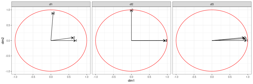<!-- --> --- ## How to interpret PCA? <iframe width="720" height="480" src="img/pca-animation.mp4" align="middle" frameborder="0" allowfullscreen></iframe> --- ## How to choose a number of PCs? .center[<img src="img/choix-nombre-composantes.png">] --- ## Using PCA as a quality control cool .center[<img src="img/design-messy.png" width="400"> <img src="img/design-tidy.png" width="400">] --- class: center, inverse, middle <!-- Section 8: Clustering --> ## Clustering --- ## Purpose of clustering Purpose: group individuals that look alike -- Depends on: * the number of groups * what "look alike" means (distance choice) -- Here: two types of clustering (HC and `\(k\)`-means) --- ## Hierarchical (Agglomerative) Clustering (HC) Is based on: * a **distance** between individuals (usually, Euclidean distance) -- * **linkage** (distance between groups of individuals): common linkage is Ward's linkage --- ## Hierarchical (Agglomerative) Clustering (HC) Is **iterative**: 1. each individual is a group 2. find the two closest group and merge them in a new group (for Ward's: minimize loss of within-group variability) 3. end when there is only one group with all individuals --- ## HC representation: dendrogram <iframe width="720" height="480" src="img/dendogramme-animation.mp4" align="middle" frameborder="0" allowfullscreen></iframe> --- ## HC representation: reading the dendrogram Distances between individuals are read following branches: .center[<img src="img/dendogramme-figure2.png">] --- ## `\(k\)`-means .center[<img src="img/K-means.png" width="1000">] --- ## Differences between the two methods * HC provides a solution for any number of clusters but can be very difficult to use if `\(n\)` is large * `\(k\)`-means requires that the number of clusters is chosen in advance but it is fastest * `\(k\)`-means is stochastic: it gives different solutions at each run depending on the initialization * HC with Ward's linkage can be seen as an approximate solution of the "best" `\(k\)`-means **In practice**: if you can, use HC first and initialize `\(k\)`-means with HC results. --- ## Credits Heavily inspired from **Sébastien Déjean**'s previous version of the class. With ideas taken from http://r-graph-gallery.com/ as well (for the part on graphics) * slide 31: contingency table from Wikimedia Commons, by ASnieckus "Table of gender by major.png" * slide 46: dot plot from http://www.sthda.com/english/wiki/wiki.php?id_contents=7868 * slide 47: barplot from ggplot2 documentation * slide 48: scatterplot matrix from http://www.sthda.com/english/wiki/scatter-plot-matrices-r-base-graphs * slide 64: Galton boxes from Wikimedia Commons, by Marcin Floryan "Galton_Box.svg" and Antoine Taveneaux "Planche_de_Galton.jpg" * slide : `\(k\)`-means clustering from Wikimedia Commons, by Mquantin https://commons.wikimedia.org/w/index.php?curid=61321400